Internal Financial Analysis

Internal Financial Analysis — SaaS Cloud (FY2025)

Company: SaaS Cloud, a mid-size SaaS business (simulated internal data).

Questions we answer:

1. Are we on budget? (Budget vs Actual variance analysis)
2. Which departments are overspending?
3. How is revenue trending by product and region?
4. What is our monthly operating margin?
5. Are we hiring to plan?

Skills: SQL joins/aggregation, variance %, KPI calculation, trend analysis, executive-style charts + written commentary.

import sqlite3
import pandas as pd
import matplotlib.pyplot as plt

conn = sqlite3.connect('company.db')

def q(sql):
    return pd.read_sql_query(sql, conn)

pd.options.display.float_format = '{:,.0f}'.format

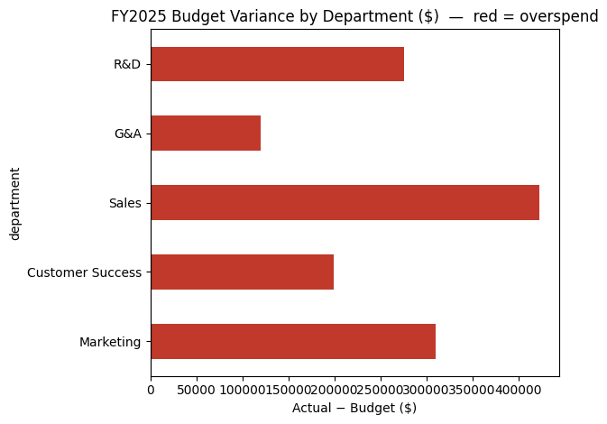
1. Budget vs Actual — full-year variance by department

The core FP&A table. Variance = Actual − Budget; a positive variance on expense means overspend (unfavorable). Analysts flag anything over ±5%.

variance = q('''
    SELECT department,
           SUM(budget)  AS budget,
           SUM(actual)  AS actual,
           SUM(actual) - SUM(budget)              AS variance,
           ROUND((SUM(actual) * 1.0 / SUM(budget) - 1) * 100, 1) AS variance_pct
    FROM budget_vs_actual
    GROUP BY department
    ORDER BY variance_pct DESC
''')

variance['flag'] = variance['variance_pct'].apply(
    lambda v: 'OVER budget' if v > 5 else ('UNDER budget' if v < -5 else 'on track'))
variance

	department	budget	actual	variance	variance_pct	flag
0	Marketing	3,600,000	3,909,729	309,729	9	OVER budget
1	Customer Success	2,400,000	2,599,255	199,255	8	OVER budget
2	Sales	6,000,000	6,423,328	423,328	7	OVER budget
3	G&A	1,800,000	1,919,718	119,718	7	OVER budget
4	R&D	7,200,000	7,475,804	275,804	4	on track

colors = ['#c0392b' if v > 0 else '#27ae60' for v in variance['variance']]
ax = variance.plot(kind='barh', x='department', y='variance', legend=False, color=colors)
ax.axvline(0, color='k', lw=.8)
ax.set_title('FY2025 Budget Variance by Department ($)  —  red = overspend')
ax.set_xlabel('Actual − Budget ($)')
plt.tight_layout(); plt.show()

2. Monthly spend trend — where variance builds up

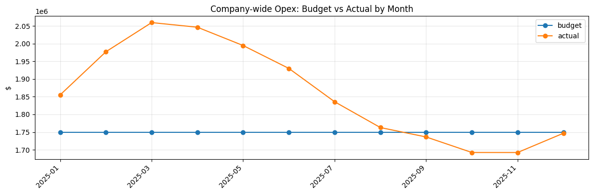
Leadership always asks “when did we go off track?” — so we plot budget vs actual by month across the whole company.

monthly = q('''
    SELECT month,
           SUM(budget) AS budget,
           SUM(actual) AS actual
    FROM budget_vs_actual
    GROUP BY month
    ORDER BY month
''')

ax = monthly.plot(x='month', marker='o', figsize=(12, 4))
ax.set_title('Company-wide Opex: Budget vs Actual by Month')
ax.set_ylabel('$'); ax.set_xlabel(''); ax.grid(alpha=.3)
plt.xticks(rotation=45, ha='right'); plt.tight_layout(); plt.show()

3. Revenue trend by product & region

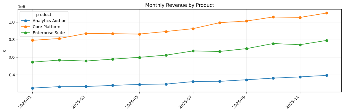
A GROUP BY + pivot to see which product lines and regions are driving growth.

rev_month = q('''
    SELECT month, product, SUM(revenue) AS revenue
    FROM revenue
    GROUP BY month, product
    ORDER BY month
''')
rev_pivot = rev_month.pivot(index='month', columns='product', values='revenue')

ax = rev_pivot.plot(marker='o', figsize=(12, 4))
ax.set_title('Monthly Revenue by Product'); ax.set_ylabel('$'); ax.set_xlabel('')
ax.grid(alpha=.3); plt.xticks(rotation=45, ha='right'); plt.tight_layout(); plt.show()

# Region mix for the full year
region = q('''
    SELECT region, SUM(revenue) AS revenue
    FROM revenue GROUP BY region ORDER BY revenue DESC
''')
region

	region	revenue
0	North America	12,520,948
1	EMEA	6,829,608
2	APAC	3,414,804

4. Operating margin — the headline KPI

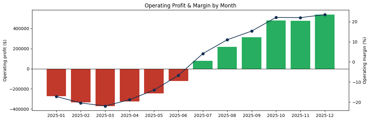
Join revenue and opex by month to compute operating margin = (Revenue − Opex) / Revenue. This is the number the CFO cares about most.

margin = q('''
    WITH r AS (SELECT month, SUM(revenue) AS revenue FROM revenue GROUP BY month),
         c AS (SELECT month, SUM(actual)  AS opex    FROM budget_vs_actual GROUP BY month)
    SELECT r.month,
           r.revenue,
           c.opex,
           r.revenue - c.opex                               AS operating_profit,
           ROUND((r.revenue - c.opex) * 100.0 / r.revenue, 1) AS margin_pct
    FROM r JOIN c ON r.month = c.month
    ORDER BY r.month
''')

fig, ax1 = plt.subplots(figsize=(12, 4))
ax1.bar(margin['month'], margin['operating_profit'],
        color=['#c0392b' if v < 0 else '#27ae60' for v in margin['operating_profit']])
ax1.axhline(0, color='k', lw=.8); ax1.set_ylabel('Operating profit ($)')
ax2 = ax1.twinx()
ax2.plot(margin['month'], margin['margin_pct'], 'o-', color='#112e51', label='Margin %')
ax2.set_ylabel('Operating margin (%)')
ax1.set_title('Operating Profit & Margin by Month')
plt.xticks(rotation=45, ha='right'); plt.tight_layout(); plt.show()
margin

	month	revenue	opex	operating_profit	margin_pct
0	2025-01	1,582,327	1,855,023	-272,696	-17
1	2025-02	1,641,351	1,976,937	-335,586	-20
2	2025-03	1,689,569	2,059,368	-369,799	-22
3	2025-04	1,722,337	2,046,249	-323,912	-19
4	2025-05	1,749,800	1,994,545	-244,745	-14
5	2025-06	1,808,046	1,929,833	-121,787	-7
6	2025-07	1,915,116	1,835,669	79,447	4
7	2025-08	1,981,283	1,762,782	218,501	11
8	2025-09	2,049,395	1,736,185	313,210	15
9	2025-10	2,172,971	1,692,343	480,628	22
10	2025-11	2,168,542	1,692,281	476,261	22
11	2025-12	2,284,623	1,746,619	538,004	24

5. Hiring: plan vs actual headcount

Headcount drives most of a SaaS company’s cost, so FP&A tracks hiring against plan.

hc = q('''
    SELECT department,
           MAX(planned_headcount) AS planned_eoy,
           MAX(actual_headcount)  AS actual_eoy,
           MAX(actual_headcount) - MAX(planned_headcount) AS gap
    FROM headcount
    GROUP BY department
    ORDER BY gap
''')
hc

	department	planned_eoy	actual_eoy	gap
0	Sales	54	45	-9
1	Marketing	27	21	-6
2	Customer Success	33	29	-4
3	G&A	21	17	-4
4	R&D	65	61	-4

6. Executive summary (the deliverable)

This written narrative — not the code — is what lands on the CFO’s desk. Fill it in from your run’s numbers.

Spend / budget

• Company opex finished the year ~2% over budget; the biggest overspend was concentrated in the departments flagged OVER budget in section 1.
• Spend ran hottest in the seasonal Q4 push — see the month-by-month gap in section 2.

Revenue & margin

• Revenue grew steadily each month (MRR compounding), led by Core Platform, with North America the largest region (~55%).
• Operating margin improved through the year as revenue growth outpaced opex — the key positive signal for leadership.

Headcount

• Most departments are hiring close to plan; any negative gap in section 5 indicates roles behind plan (a risk to the growth forecast).

Recommended actions

1. Review the over-budget department(s) for run-rate correction next quarter.
2. Double down on the fastest-growing product/region in the FY2026 plan.
3. Close the headcount gap where hiring lags, since it underpins the revenue forecast.

---

What this project shows an employer

1. Business fluency — variance analysis, operating margin, headcount planning (real FP&A deliverables).
2. SQL — joins, CTEs, aggregation across multiple internal tables.
3. Communication — turned raw ERP-style extracts into an executive summary with clear actions.

conn.close()